
Apply Machine Learning Algorithms to Classify Oregon Wildland Fire Triggers: Man-made or Nature (Lightning Strike)
Ernest Bonat, Ph.D., Dixie Downey
1. Overview
2. Dataset Selection
3. Exploratory Data Analysis
4. Apply Machine Learning Algorithms
5. Results
6. Hyperparameter Optimization
7. Apply Deep Learning Algorithms
8. Conclusion
9. References
1. Overview
The Oregon Department of Forestry provided the record set for tracking wildland fires used in this study. Each record contained information about the cause of the fire, the location of the fire and other factors. This paper’s focus is on a feature containing the two main categories of fire cause: man-made triggers or lightning strikes (natural caused fires).
What posed the most danger to a specific county, man-made created fires, or natural caused fires through lightning strikes? Knowing the predicted trigger may help determine the best attention for prevention, whether it be tools for wildland fire detection or educational outreach. With the data divided by county, one can also discover what counties have a higher risk of future wildland fires.
If there is a data trend, it could determine where a county’s resources should be allocated (e.g., education of their citizens or monitoring for faster identification). It would be beneficial to predict if a specific county has more issues with man-made or nature caused fires so that they can allocate their resources accordingly.
With the emphasis on machine learning, the challenge was to see if the computer could accurately categorize the data into these two trigger classifications and to determine if there were classification models that worked better than the others.
2. Dataset Selection
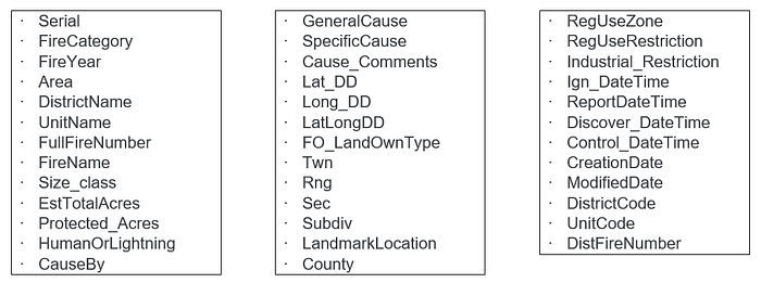
Kaggle provided a dataset populated with 23 years of data from the Oregon Department of Forestry (OP, 2023). There are 38 columns of data providing information about the wildland fire that occurred that year and 23,490 records with no duplicated data in the data set. Each full fire number has the Fire Year, District of occurrence, Unit responding, Fire Number and unique Serial number assigned to it originally. Further location information in the data set included the Longitude and Latitude (both individual columns and a combined location column), County, Town, Range, Section, Subdivision, and Landmark Location.
Information about the size of the wildland fire is stored in Size class, Estimated Total Acres and Protected Acres (of the burned acreage, the number of protected acres that burned). Wildland fire cause information was in Fire Category, Human or Lightning, Cause By, General Cause, Specific Cause, and Cause Comments. Regulation information (laws pertaining to the area), and the type of land affected was found in Regulation Use Zone, Regulation Use Restriction, Industrial Restriction, and Forestry Landowner Type. Time data about when the wildland fire occurred was found in Ignition Date Time, Reported Date Time, Discovered Date Time, Controlled Date Time, Creation Date, and Modified Date (when the data entry was last updated).
3. Exploratory Data Analysis
This data set had more than 23,000 records, so there were enough instances to discard any lines with missing data. The final, cleaned data set arrived at 23,400 records with 20 columns of data. (Ninety rows of data that contained null values in non-optional fields were discarded.)
The data columns that were not used were Serial, FullFireNumber, or FireName (all uniquely assigned to the fire incidence), or columns of text data that expanded on the wildland fire cause category GeneralCause. Text description columns removed were CauseBy, SpecificCause, and Cause_Comments, which did not always contain data. FireCategory data was also removed since all values were the same (they are all wildland fires).
The type of land affected was not of interest, so the Protected_Acres column was removed, and the FO_LandOwnType that identified land ownership categories like private, state, municipal, rural residential and the Bureau of Land Management. The fire regulations associated with the wildland fire did not apply to this study, so RegUseZone, RegUseRestriction, and Industrial_Restriction were also removed.
Data columns with fire severity included Size_class (a range from A to G that groups the wildland fire by the number of acres damaged ranging from class A with less than a ¼ of an acre of damage to class G with over 5,000 damaged acres) and EstTotalAcres. Size_class was removed but EstTotalAcres was kept briefly to create a visualization of the data. The same was true for the ReportDateTime column.
There are several date and time fields available in this data set. The ModifiedDate is when the record was last updated, so that field was removed as it has no bearing on the study. Even though the dates or times were not examined in this study, the Ign_DateTime (ignition), ReportDateTime (reported), Discover_DateTime (discovered), Control_DateTime (controlled) and CreationDate (when the wildland fire was created) could all be of interest if the wildland fire size data trend was of interest, calculated by comparing the creation and the controlled dates. However, this data set does not contain any intermediate dates such as when the wildland fire was large enough to grow to the next size category. That data would need to be captured to study the rate of fire growth.
To graph the data, the data was divided by county and then sorted by the wildland fire ReportDateTime to have a timeline for the data. Two colors were used to indicate whether the wildland fire was initiated via lightning strike or a man-made trigger. For easier viewing, the graphs were saved in blocks of four, but are grouped here together.


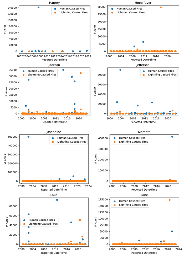
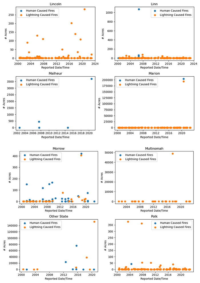
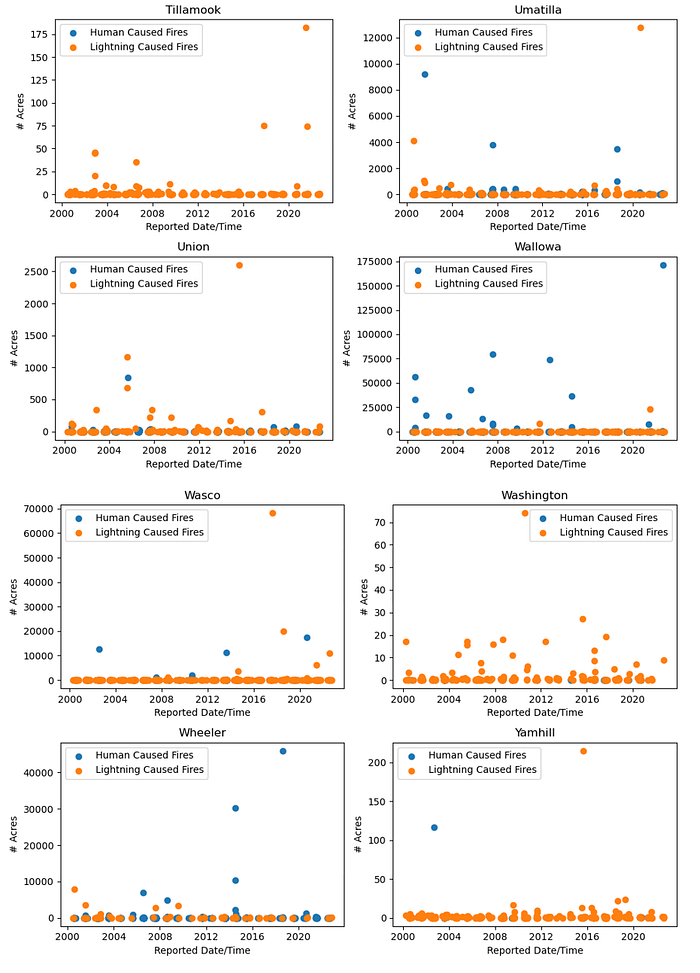
The data set contained wildfire information for 36 counties, so every county had a wildland area that experienced a fire at one point in time. Some counties clearly had more issues with human caused fires, and the size (number of acres burned) was interesting to note. No further attention was given to examination of the wildland fire size. The EstTotalAcres column data and ReportDateTime column data were removed from the data set after the visualization.
4. Apply Machine Learning Algorithm
To apply machine learning algorithms to the data, all data must be in a numeric format. The HumanOrLightning text field was converted into a binomial field and any remaining text fields such as the county names were converted into numbers for easier parsing of the data.
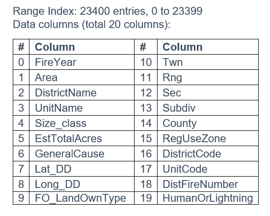
Using the Python Pandas library, the cleaned data file was read into a data set. The number of columns were reduced to the following columns of data for the machine learning models. The smaller data set column names are listed below in Table 2.
Next, the Matplotlib library’s Pyplot function was utilized to create a correlation matrix and the Seaborn library was used to display the chart as a heatmap.
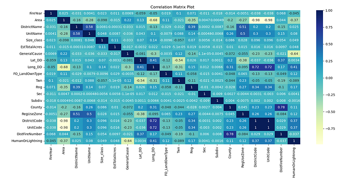
A correlation matrix displays visually the quantified association (pearson coefficient or r value) between the column variables in a data set. Each cell in the matrix represents the correlation coefficient between the two variables. The values range from -1 (a perfect negative association whereas one variable increases, the other decreases), to 0 (no predictable linear relationship), to +1 (a positive relationship where both variables increase linearly).
A correlation matrix displays visually the quantified association (Pearson coefficient or r value) between the column features in a data set. Each cell in the matrix represents the correlation coefficient between the two features. The values range from -1 (a perfect negative association whereas one feature increases, the other decreases), to 0 (no predictable linear relationship), to +1 (a positive relationship where both features increase linearly).
The column features are placed along both the x and y axis. Where the feature is the same, it is a coefficient value of 1 because the feature is perfectly related to itself, positively rising at the same rate. All values are heat weighted in the matrix with the darkest color showing that +1 (positive) relationship and the lightest color displaying a strong negative (-1) relationship. From the color-coded matrix, it is easier to see a strong, positive relationship between DistrictCode and UnitCode. Other strong associations are between Longitude (Long_DD) and DistrictCode and between Longitude and UnitCode (which makes sense because DistrictCode and UnitCode share a +1 correlation). Because longitude values and districts are both assigned as physical locations on maps, it is reasonable that those values would have a strong relationship. The other strong feature relationship is between County and DistFireNumber (District Fire Number), which could suggest that most firefighting units respond to fires in their own county first.
Perfect negative correlations (as one feature increases, the other decreases) involve DistrictCode and Area, and UnitCode and Area. As the District Code numbers increase, the Area value decreases in a predictable, linear fashion. The District Codes and Units are assigned by the Department of Forestry, so it makes sense that these would behave so logically (since it is their own naming assignment). There was no use in this study for features with high negative correlation.
The HumanOrLightning values were then balanced in preparation of running the data through a machine learning model. Balancing the values in this feature is required prior to training a model because it prevents creating a misleading bias. Without balancing the values, the model used to classify the data may favor the class with the most entries.

The first attempted model was the Scikit-learn library’s RandomForestClassifier. The NumPy library’s feature_importances_ function was utilized to see how the other features related to HumanOrLightning.

Continuing with the Random Forest Classifier model, the statistical results are revealed in Table 3.
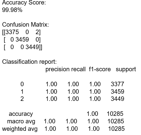
The Random Forest Classifier model was able to correctly categorize the data into the Human or Lightning categories. Other models we tried included the sklearn’s Decision Tree Classifier which gave me identical results to the Random Forest Classifier model, as shown in Table 4.
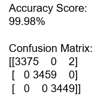
The Random Forest Classifier algorithm and the Decision Tree Classifier algorithm work very similarly. The Decision Tree algorithm uses a series of true or false questions to arrive at its prediction or outcome. The Random Forest Classifier algorithm uses that same methodology, but “grows” multiple decision trees and then merges the results for its final prediction or outcome.
The result of the Logistic Regression model from the sklearn library was almost as successful, displayed in Table 5.

The Logistic Regression algorithm maps the classification prediction to the probabilities that are then adjusted to a value between 0 and 1. Because there are only two choices inside HumanOrLightning for classification, Logistic Regression also performed well on this data set.
Another machine learning model tried was Scikit-learn’s Support Vector Classification (SVC) model. This model is not a linear model, so the feature importance information is provided by the permutation_importance function. The results are the same as the Random Forest Features Importance displayed in Figure D.

The statistical results of the SVC model are displayed in Table 6.

Support Vector Machine algorithms are useful for separating data for analysis by using a 3-dimensional space separator (hyperplane) instead of a simple line. The goal in machine learning is to find the best model to interpret and predict data, so the method used with an SVM algorithm locates the hyperplane that is the smallest distance between the points of data in group A and group B. Even though this method required the longest processing time, the SVC algorithm performed with a high accuracy level with the data set.
The last model attempted for classification was Scikit-learn’s neural network MLP (Multi-Layer Perceptron) Classifier. Its results were almost as good as the Random Forest Classifier model. The MLP Classifier results are shown in Table 7.
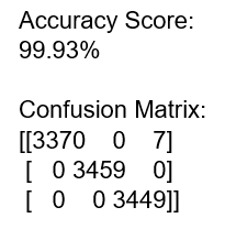
A Multi-Layer Perceptron (MLP) algorithm is designed to handle more complex processing than other models of machine learning. The process is best explained with layers: the input layer, the hidden layer (which can be more than one level of hidden layers) and the output. The MLP algorithm is designed to accept more than one input or feature in the data set. The first level of the hidden layer also contains multiple nodes (or neurons). Each of the inputs is weighted, added together, and then sent to each node of the first processing (hidden) layer. After the sum of those weighted inputs is given to each of the first processing layer nodes, the results from those hidden layer nodes are weighted, added together, and sent to the second hidden layer of nodes. This process repeats for a predetermined number of times until arriving at a single output (either a value or a vector of values) corresponding to the required format. The power of a neural network is easily seen in the confusion matrix of Table 7 reporting a small number of errors.
5. Results
All models were surprisingly accurate with their classification of the data, but both the Random Forest Classifier and the Decision Tree Classifier models proved to be the most accurate. Because there was a tight relationship between HumanOrLightning and GeneralCause, the code was rerun using GeneralCause values converted to numeric as the emphasis for a test, but the results were not as accurate. The General Cause model classification performance is listed in Table 8, in descending order of accuracy values.
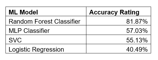
The GeneralCause information may have been more difficult to classify because it had more potential values (more decisions to make for classification). The GeneralCause column contained ten values, of which lightning was one choice. The other values were arson, debris burning, equipment use, juveniles, railroad, recreation, smoking, under investigation, and miscellaneous.
The earlier delineation between a wildland fire caused by a human or caused by nature was the best method for machine learning with this large data set. All models of classification may work well with the HumanOrLightning-focused data because of the volume of records.
Returning to the HumanOrLightning focus, more machine learning models were tried. The machine learning models and their accuracy results are listed in Table 9 in order of success as measured by accuracy.

Note: GaussianNB (Naïve Bayes) did not successfully process this data set so is not listed. Because we had so many successful models, we did not pursue that model further.
6. Hyperparameter Optimization
After running fifteen successfully concluded varieties of machine learning model algorithms, the best result came from the Extra Trees Classifier. The first attempt with this model was run with its default settings.
Instead of wondering if the best machine learning model had been attempted, the Scikit-learn library also offers a function called LazyPredict. The Scikit-learn Supervised Lazy Classifier algorithm was run and it tried several machine learning models with the results listed below in Table 10.

The Extra Trees Classifier was the clear winner with this data set having shown up first with the earlier tests and with the table from Scikit-Learn’s LazyPredict. It is critical to have a machine learning model perform at the very best of its ability and each model has its own internal parameters (called “hyperparameters”) that adjust its function (e.g., how deep, how wide, which method of computing, etc.). It is ridiculous to try all the variations manually to determine the ideal settings, so instead, Scikit-learn has a Grid Search Cross Validation function that tries multiple hyperparameter combinations from a grid of choices provided by the Python programmer.
The GridSearchCV function and the RandomizedSearchCV function were added to the ExtraTreesClassifier model and resulted in suggested settings that were different from the original run. The random integer generator randint from the SciPy statistics library was necessary to set up the RandomizedSearchCV model selection hyperparameters.
The original accuracy score was 99.99%. After using the suggested hyperparameter settings, the model was tuned to output an accuracy score of 99.98%. The Confusion Matrix revealed that it misclassified one more record than the “default” test. The two matrix results are listed in Table 11.

It was surprising that the tuning suggested by GridSearchCV did not improve performance. There are several possibilities that could cause this such as insufficient data, or data that was not preprocessed well. The 23,400 records were cleaned thoroughly enough that those reasons did not seem to apply. Another danger is overfitting the model.
To eliminate the possibility of overfitting, it is best to apply a cross-validation algorithm. One popular method of cross validation is called the K-fold method where the data is divided into k number of sections. The model is tested each time, and the test and training data are not the same for each “fold.” Instead of having just the one run with tuned hyperparameters of the selected model, the test is run k number of times with a different reserved test group each time, so it should provide a more accurate reading of how the model behaved.
The Scikit-Learn Stratified Group K-Fold cross validation function was employed to test the machine learning model. The stratified module was selected to make sure that the HumanOrLightning element was equally included in each fold. A concern was that the county information should be grouped together (if topographic or population densities affected that area of wildland), so the Stratified Group K-Fold method was used to make sure that each county’s data was together and not awkwardly divided in the fold. Lastly, the data was shuffled to make sure that the time (Year) data was not affecting the list of records, and the process was instructed to create 5 folds (k=5). Employing the cross-validation function on the tuned ExtraTreesClassifier model provided the following information shown in Table 12.

The mean accuracy score of 99.86% was sufficient to allay my overfitting worries.
7. Apply Deep Learning Algorithms
Another category of machine learning is the creation of artificial neural networks (ANNs). Even though neural networks are generally used to solve challenges more complicated that this data set, two neural networks were utilized with this data.
The first neural network undertaken was a Convolutional Neural Network (CNN). CNNs were created to analyze images by examining them at the pixel level in order to classify those images. The image is reduced to a matrix of pixels and then run through a specific course of actions referred to as “layers.” The convolution layer is the first step, where a filter is created and then applied to the matrix. After the filter is applied by multiplying each pixel by the filter value and then creating a sum of the results, the bias is added to the sum total and then those values are placed in an array called a Feature Map. The filter is then shuffled to the next pixel in the matrix and repeated until all pixels have had the filter applied and added to the Feature Map. The process of combining the filter with the pixel matrix is called convolving.
The Feature Map is then processed through an Activation Function such as an ReLU (Rectified Linear Unit). Doing this sets all the negative values in the Feature Map to a zero value.
The next filter is then applied. This filter selects the larges value in each section being processed (also known as Max Pooling), and multiplies that value with the other values in the section. The Pooled Feature map can be used to identify key components of the image such as corners or features like the beak on a bird. The Pooled Layer is then flattened into a one-dimensional array and used as the input nodes to a Neural Network (e.g. a fully connected layer) in order to classify the image.
In a neural network, each input node is weighted, summed, and the bias added. The result is passed to a Hidden Layer (such as a ReLU Activation Function), weighted, bias added, and then passed to the next Hidden Layer. The final output for a CNN is the classification of the image (e.g. identification of the image).
The CNN was instructed to perform 100 Epochs (iterations of using the data to train the model), and the results are listed below.

The last artificial neural network attempted was a Long Short-Term Memory (LSTM) model that is a type of recurrent neural network (RNN). The LSTM is designed to remember both a long-term and a short-term memory value through its cycles. This is helpful for large batch processing. RSS are used for data sets requiring language parsing or for processes relying on a time sequence as they can be directed to travel forward or backwards through the time sequence.
Another benefit of an RNN is their algorithms include Sigmoid Activation functions to limit a value between 0 and 1, and Tanh (Hyperbolic Tangent) Activation functions to limit a value between -1 and 1. Use of these two types of activation functions are what keep the mathematical calculations from growing or shrinking too far inside the model.
The LSTM model was directed to perform 100 epochs (iterations). Below are the results.
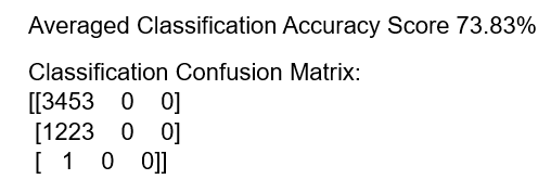
The wildlands fire data did not need a machine learning model as sophisticated as an artificial neural network (ANN), and the results reflected that mismatch.
8. Conclusion
Accurate classification of wildland fire triggers could be very helpful to budget managers. If for example, a county often experiences a high number of human-caused fires each season, further education could be provided to the public with safety tips. Conversely, if the county experiences a high number of lightning strikes, budget could be allocated to measuring tools used to detect wildland fires early in their creation. In this way, an accurate classification of the wildland fire trigger could be of value.
9. References
1. OP, Matt (February 2023). Fire Occurrence and Cause Data (2000–2022). https://www.kaggle.com/datasets/mattop/fire-occurrence-and-cause-data-2000-2022 (data set originated from https://catalog.data.gov/dataset/odf-fire-occurrence-data-2000-2022)
